Research
Neutrino phenomenology
Neutrino phenomenology · Particle physics beyond the Standard Model · Astroparticle physics · Cosmology
Research statement
Overview
I have been a researcher in theoretical physics from 2005 to 2015 and associate professor until 2023. I am currently Full Professor of Theoretical Physics at the University of Bari "Aldo Moro".
My research lies at the interface between neutrino physics, particle phenomenology and cosmology. With the Bari group I have contributed to a long line of global analyses of neutrino oscillation data, combining solar, atmospheric, reactor and accelerator experiments to extract the fundamental parameters of leptonic mixing with state-of-the-art precision.
As measurements enter the subpercent regime, these results sharpen the picture of the neutrino mass ordering, of leptonic CP violation and of the absolute neutrino mass scale, while probing possible signatures of physics beyond the three-neutrino paradigm.
Where this work sits
Full Professor of Theoretical Physics, Università degli Studi di Bari “Aldo Moro” and INFN Sezione di Bari. Researcher from 2005, associate professor to 2023.
Research theme 01
Global analysis of neutrino oscillations
Three-flavour fits to the world neutrino data, with a self-consistent treatment of solar, atmospheric, reactor and long-baseline accelerator experiments.
The observables are the two mass-squared splittings $\Delta m^2_{21}$ and $|\Delta m^2_{3\ell}|$ and the three mixing angles $\theta_{12}$, $\theta_{13}$, $\theta_{23}$ of the PMNS matrix, together with the CP-violating phase $\delta_{\rm CP}$. In vacuum the survival probability of a flavour eigenstate takes the familiar form
$$ P(\nu_\alpha \to \nu_\alpha) = 1 - 4\sum_{i<j} |U_{\alpha i}|^2 |U_{\alpha j}|^2 \sin^2\!\left(\frac{\Delta m^2_{ij} L}{4E}\right), $$but the precision now attainable requires the full matter-effect treatment and a careful statistical combination of datasets with very different systematics.
Interactive figure
Three-flavour oscillation lab
Exact coherent three-flavour vacuum oscillations. The amplitude is summed over the mass eigenstates with the complex PMNS matrix and only then squared, so no curve is an independent sine wave and the three sum to one at every point.
A(να→νβ) = Σi Uβi exp[−i · 2.534 · Δm²i1 · L/E] U*αi
P(να→νβ) = |A(να→νβ)|²
L in km, E in GeV, Δm² in eV². The three amplitudes are evaluated as complex numbers and only then squared, so no curve is an independent sine wave.
Parameters in use
- sin²θ12
- 0.303
- sin²θ13
- 0.0223
- sin²θ23
- 0.473
- δCP
- 1.20 π
- δm²
- 7.37 × 10⁻⁵ eV²
- Δm²
- 2.495 × 10⁻³ eV²
- Δm²31
- —
- ordering
- normal
Every value above is our own, from Table I of Phys. Rev. D 111, 093006 (arXiv:2503.07752), in this group's conventions: δm² = m2² − m1² and Δm² = m3² − (m1² + m2²)/2. They are not NuFIT's Δm²3ℓ and cannot be compared with it at a glance, which is why Δm²31, the splitting the phases actually need, is derived here rather than quoted: Δm²31 = Δm² + δm²/2. Normal ordering throughout — the same analysis favours it at 2.2σ. Propagation is parameterised by L/E; the scan is a way of reading the curve, not physical time.
Interactive figure — detector response
Water-Cherenkov event
The neutrino emits no Cherenkov light: it is neutral, it crosses the water unseen, and its direction is only inferred after the fact. Light appears when the charged lepton produced at the vertex travels faster than the phase velocity of light in water, c/n, which is well below c. The cone opens at cos θC = 1/(βn), and its intersection with the sensor wall is the ring.
State
- βn
- —
- cos θC
- —
- θC
- —
- stage
- —
- hit PMTs
- —
Nothing here moves faster than light in vacuum. The charged lepton exceeds only c/n, the phase velocity of light in water, which is why the wavefronts pile up into a cone; below βn = 1 the condition fails and no light is produced. Distances are schematic and the sequence is paced for reading, not to scale in physical time.
Current best fits
The six parameters, as we measure them
What the global analysis returns for the three mixing angles, the two mass-squared splittings and the CP phase — the quantities every figure above is drawn from.
Normal-ordering best fits from Capozzi, Giarè, Lisi, Marrone, Melchiorri and Palazzo, Phys. Rev. D 111, 093006 (2025), Table 1; δm² = m₂² − m₁², Δm² = m₃² − (m₁² + m₂²)/2. NO is favoured over IO at 2.2σ. The 1σ precision is one sixth of the 3σ range.
Research theme 02
Mass ordering and leptonic CP violation
Statistical extraction of the leptonic CP phase $\delta_{\rm CP}$ and of the sign of $\Delta m^2_{3\ell}$ from the interplay of T2K, NOvA, reactor and atmospheric data. The two datasets pull in partly different directions, and the resulting significance depends delicately on how their systematics are combined.
A related strand is forecasting the discovery reach of the next generation of experiments — JUNO, DUNE and Hyper-Kamiokande — and identifying which combinations of measurements would resolve the ordering and the $\theta_{23}$ octant with the least model dependence.

Interactive figure · JUNO · reactor antineutrinos at 52.5 km
How a reactor 52.5 km away reads the mass ordering
The reactor antineutrino spectrum at JUNO, built up one ingredient at a time: the slow solar oscillation, the fast atmospheric ripple on top of it, the phase shift that tells normal from inverted ordering, and what detector resolution and statistics leave of it. Step through the seven scenes, or take the controls yourself.
Step 1 / 7
Reactor antineutrinos
Fission in the reactor cores emits ν̄e up to about 10 MeV. JUNO detects them through inverse beta decay, and flux times cross section gives a spectrum that peaks near 3 MeV of visible energy.
Switch NO ↔ IO and watch the fast ripple slide in phase — more at low energy than at high.
No smearing: every ripple is resolved.
100%
RMS of the NO − IO difference (lower panel), relative to perfect resolution.
P(ν̄e→ν̄e) = 1 − cos⁴θ13 sin²2θ12 sin²Δ21 − sin²2θ13 (cos²θ12 sin²Δ31 + sin²θ12 sin²Δ32), Δij = 1.267 Δm²ij[eV²] L[m] / E[MeV]
Bari global analysis: δm² = 7.48×10⁻⁵ eV², sin²θ12 = 0.3085 (Phys. Rev. D 114, 016026); sin²θ13 = 0.0223, Δm² = 2.495×10⁻³ eV² (NO; Phys. Rev. D 111, 093006), with δm² = m₂² − m₁² and Δm² = m₃² − (m₁² + m₂²)/2. IO is drawn with the same effective Δm²ee = cos²θ12|Δm²31| + sin²θ12|Δm²32| as NO, as a fit would choose it, so the difference that remains is the ordering alone. Flux: Mueller et al. (2011) with fission fractions 0.58, 0.07, 0.30, 0.05 (²³⁵U, ²³⁸U, ²³⁹Pu, ²⁴¹Pu); inverse-beta-decay cross section at leading order; Evis ≈ Eν − 0.78 MeV. Single baseline, no backgrounds, no systematics; pseudo-data drawn with a fixed random seed.
Research theme 03
Absolute neutrino masses and cosmology
Oscillation experiments are sensitive only to mass-squared differences. The absolute scale is constrained instead by three complementary probes: the endpoint of the β-decay spectrum, which measures the effective mass $m_\beta$; searches for neutrinoless double-β decay, sensitive to the Majorana mass $\langle m_{\beta\beta} \rangle$; and cosmological observations of the CMB and of large-scale structure, which bound the sum $\Sigma = \sum_i m_i$.
Combining these with the oscillation results is a genuinely statistical problem, since the three observables depend on different combinations of the same underlying parameters and carry very different systematics. Our analyses map the allowed regions in the $(m_\beta,\ \langle m_{\beta\beta}\rangle,\ \Sigma)$ space, and quantify how the tension between cosmological bounds and laboratory limits evolves as data improve.
Current bounds
Where the absolute scale stands
The three probes, as they constrain the scale today — one laboratory limit each from β decay and from neutrinoless double-β decay, and the cosmological sum.
Cosmology · relic neutrinos
The cosmic neutrino background
from the primordial plasma to today
Stage 1 / 4 · thermal equilibrium
10.00MeV
≈ 0.01 s
—
Thermal equilibrium
—
Comoving temperature aT
Annihilating pairs heat the photons and not the decoupled neutrinos. That gap is the whole content of (4/11)1/3.
Momentum distribution
In comoving variables the shape is frozen. What changes is the physical scale: —
Tγ
—
Tν
—
Tν/Tγ
—
scale factor a
—
Γν/H
—
epoch
—
- Standard ΛCDM background with three light active neutrinos and no extra relativistic species.
- Decoupling is not an instant. The estimate Γν/H ≈ (T/1.4 MeV)³ only locates where the two rates cross; the transition is spread over roughly 3 to 1 MeV, is momentum dependent, and differs by flavour because νe keeps its charged-current channel slightly longer.
- The ratio (4/11)1/3 assumes decoupling completed before e± annihilation. Solving the full kinetic equations gives small distortions to the Fermi–Dirac spectra instead.
- Neff ≈ 3.044 parameterises the total radiation density relative to one instantaneously decoupled species. It is not a count of particles and not a count of flavours; the shift above 3 comes from residual heating during annihilation, flavour oscillations and finite-temperature QED corrections.
- Neutrino masses are neglected in the thermal history. They matter for the present energy density and for structure formation, not for the temperature relations shown here.
- The quanta on screen are a schematic census of a few dozen particles, not a simulation, and animation speed is a reading pace with no relation to cosmic time.
Research theme 04
Supernova neutrinos
Flavour evolution in the one place where neutrinos are dense enough to refract off each other.
A core-collapse supernova releases almost all of its gravitational binding energy as neutrinos, and it does so before anything is visible at the surface. They leave the collapsing core while the shock is still buried, which makes them the only messengers that carry direct information about the proto-neutron star and about the mechanism that revives the explosion. SN 1987A remains the sole detection: a couple of dozen events, and still the observational basis of most of what can be said. The next galactic supernova will be recorded by detectors that did not exist then, and the question is what those events can be made to say.
What makes the problem hard — and what our work has been about — is that the neutrino flux near the core is dense enough that neutrinos refract off each other. The flavour evolution stops being a one-particle problem and becomes a non-linear, collective one: the state of the ensemble enters the Hamiltonian that evolves it. With the Bari group we studied how these collective flavour transitions behave once the geometry is treated honestly rather than in a single-angle approximation, and how the multi-angle structure of the emission changes the outcome; how the transitions look when all three flavours evolve together instead of two; and how the resulting spectral splits depend on the relative luminosities of the species. We also worked out the consequences for the low-energy end of the spectrum in inverted ordering, and, more recently, on classifying the fast flavour conversions — instabilities that develop on scales far shorter than the ones set by the mass splittings — through the dispersion relation of the flavour field.
Selected work
Papers on collective flavour transitions
-
Fast flavor conversions of supernova neutrinos: classifying instabilities via dispersion relations
Phys. Rev. D 96, 043016 (2017) arXiv:1706.03360
-
Supernova neutrinos and antineutrinos: ternary luminosity diagram and spectral split patterns
JCAP 10, 002 (2009) arXiv:0907.5115
-
Supernova neutrino three-flavor evolution with dominant collective effects
JCAP 04, 030 (2009) arXiv:0812.3031
-
Low-energy spectral features of supernova (anti)neutrinos in inverted hierarchy
Phys. Rev. D 78, 097301 (2008) arXiv:0808.0807
-
Collective neutrino flavor transitions in supernovae and the role of trajectory averaging
JCAP 12, 010 (2007) arXiv:0707.1998
Educational visualization · configurable templates
A galactic supernova in neutrinos
Two example emission templates are supplied below. Neither is a prediction: both are illustrative shapes with uncertainty bands, kept in a replaceable data object so that real collaboration output can be dropped in. What the figure is for is the structure of the burst in time and energy, and the way different detector technologies see different flavours of it.
—
1 · Collapsing stellar core
2 · Emission timeline
arbitrary normalized units
3 · Energy–time map
model dependent · arb. units
4 · Detector response
Liquid argon
—
—
- The two templates are illustrative shapes with uncertainty bands, not predictions. Progenitor mass, equation of state, rotation, the treatment of neutrino transport and the onset of explosion all change the luminosity and mean-energy histories.
- Phase boundaries are approximate. The breakout burst, the accretion phase and the cooling phase overlap, and their durations differ between simulations.
- Flavour conversion in a supernova is not settled. MSW resonances in the stellar envelope, collective neutrino–neutrino refraction, fast flavour instabilities, matter turbulence, shock passage and the unknown mass ordering can all reshape the flavour composition that arrives at Earth.
- νx here stands for the heavy-lepton flavours as a single effective species, as most templates report them.
- Event totals are deliberately not compared between technologies. That comparison is only meaningful once mass, target composition, threshold, efficiency, distance and channel cross sections are all specified; this figure fixes none of them.
- The 1/d² scaling is applied to the displayed relative rate. With normalized templates the vertical axis stays in arbitrary units; supply absolute fluences in the data object to obtain physical counts.
- Animation time is a reading pace. The horizontal axis is post-bounce time, but the playback rate is not real time.
Research theme 05
Beyond the three-neutrino paradigm
Tests of the standard 3ν framework against possible extensions.
The three-neutrino picture describes the data remarkably well, but it is not guaranteed to be complete. We test it against light sterile states, which would appear as additional mass-squared splittings and mixing angles; against non-standard neutrino interactions, which modify the matter potential and therefore the effective mixing in the Sun and in the Earth; and against tensions among datasets, which — if they persist as statistics grow — may be the first indication of new physics rather than of underestimated systematics.
Research theme 06
Modular invariance and the flavour puzzle
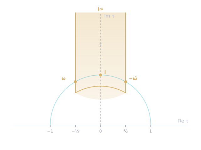
Following the proposal by F. Feruglio that the Yukawa couplings of leptons could be modular forms of a complex modulus $\tau$ living in the upper half-plane, modular invariance has emerged as a powerful candidate symmetry for the flavour structure of quarks and leptons.
With G.-J. Ding (USTC), E. Lisi (INFN Bari) and S. T. Petcov (SISSA/IPMU) we have carried out the first joint fit of quark and lepton observables — 22 quantities in total — within a modular flavour model based on the binary octahedral group $2O$, with just 14 real parameters. The fit reveals strong correlations among observables, notably between quark mass ratios and the leptonic CP phase $\delta_{\rm CP}$, that are invisible in separate analyses and that translate into sharp predictions for KATRIN, neutrinoless double-β decay, JUNO and DUNE.
In a complementary direction, with F. Feruglio (Padova), A. Strumia and A. Titov (Pisa), we have shown that modular invariance can also address the strong CP problem in string-inspired settings, where quarks have positive modular weights and gauge kinetic functions are non-trivial.
Selected recent publications
The complete list is maintained on INSPIRE-HEP.
-
Solving the strong CP problem in string-inspired theories with modular invariance
JHEP 08 (2025) 076 arXiv:2505.20395
-
Interplay and correlations between quark and lepton observables in modular symmetry models
Phys. Rev. D 111, 075024 (2025) arXiv:2409.15823
-
Neutrino masses and mixing: entering the era of subpercent precision
Phys. Rev. D 111, 093006 (2025) arXiv:2503.07752
-
Unfinished fabric of the three neutrino paradigm
Phys. Rev. D 104, 083031 (2021) arXiv:2107.00532
-
Current unknowns in the three neutrino framework
Prog. Part. Nucl. Phys. 102, 48 (2018) arXiv:1804.09678
-
Global constraints on absolute neutrino masses and their ordering — Addendum
Phys. Rev. D 101, 116013 (2020)
NOW — Neutrino Oscillation Workshop
Otranto, biennial. One of the longest-running European workshops in neutrino physics, gathering theorists and experimentalists for in-depth discussions on the frontiers of the field. I am among the organizers.
For prospective students and postdocs
I welcome motivated students and young researchers interested in neutrino phenomenology, statistical analysis of particle physics data, and the interplay between particle physics and cosmology.
A historical note
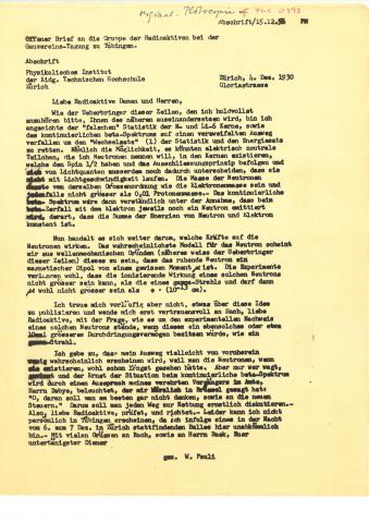
Pauli’s letter, 1930
The story of neutrinos began with one of the most famous letters in twentieth-century physics. On 4 December 1930 Wolfgang Pauli postulated a new neutral particle of tiny mass to rescue energy conservation in β-decay — a hypothesis he himself called “a desperate remedy”.
Dear Radioactive Ladies and Gentlemen, as the bearer of these lines will explain to you in more detail, because of the “wrong” statistics of the N and Li⁶ nuclei and the continuous beta spectrum, I have hit upon a desperate remedy to save the “exchange theorem” of statistics and the law of conservation of energy. Namely, the possibility that there could exist in the nuclei electrically neutral particles, that I wish to call neutrons, which have spin ½ and obey the exclusion principle and which further differ from light quanta in that they do not travel with the velocity of light. […]
But only the one who dare can win, and the difficult situation, due to the continuous structure of the beta spectrum, is lighted by a remark of my honoured predecessor, Mr Debye, who told me recently in Bruxelles: “Oh, it is best not to think about this at all, like new taxes”. […]
Unfortunately, I cannot appear in Tübingen personally since I am indispensable here in Zurich because of a ball on the night of 6/7 December. With my best regards to you, and also to Mr Back.
Your humble servant, W. Pauli.