Interactive neutrino physics · Mass ordering
How can a reactor 52.5 km away tell the neutrino mass ordering?
The reactor antineutrino spectrum at JUNO, built up in seven scenes: the slow and the fast oscillation, normal against inverted ordering, and what energy resolution and statistics leave of the difference.
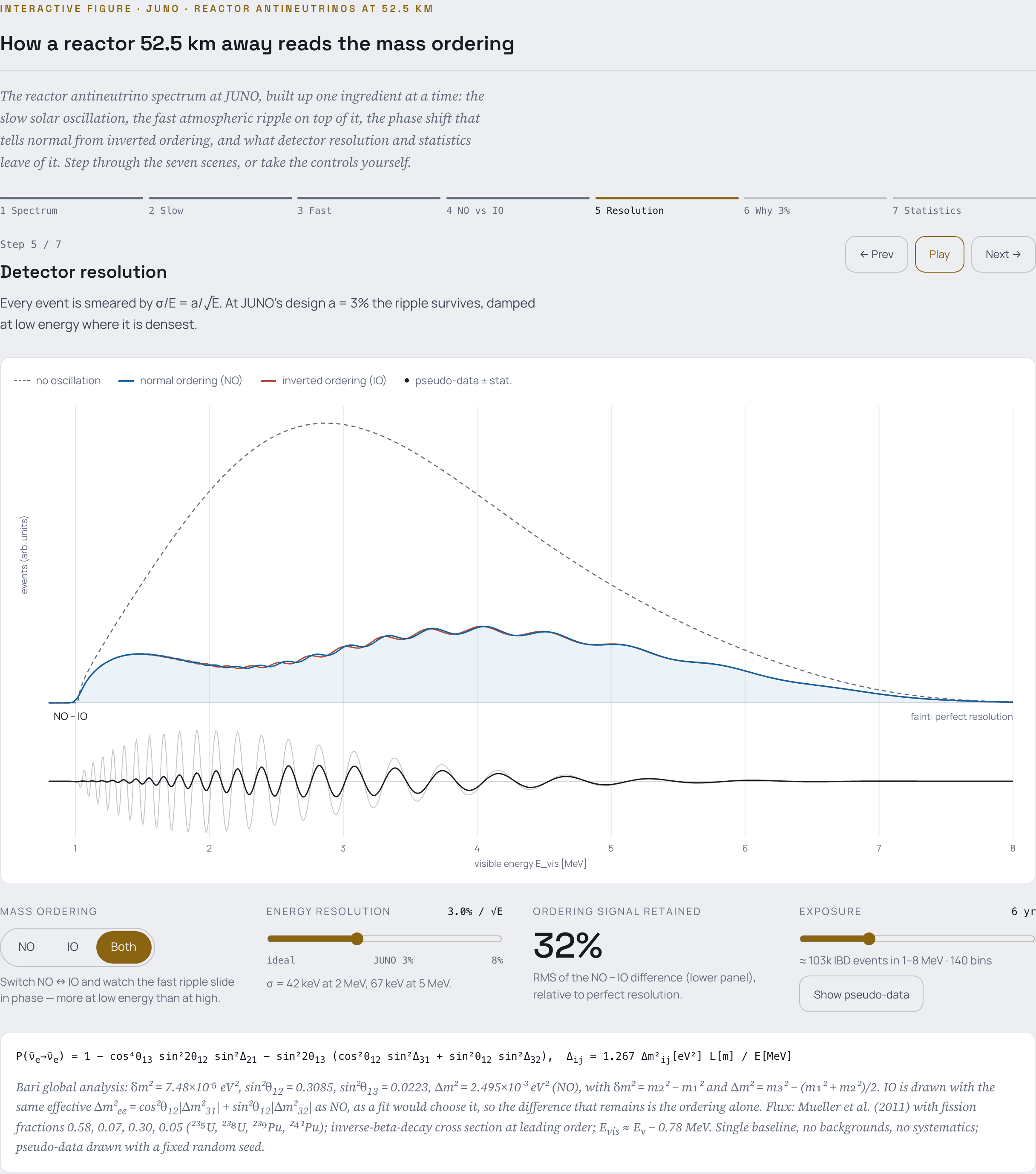
Interactive figure · JUNO · reactor antineutrinos at 52.5 km
How a reactor 52.5 km away reads the mass ordering
The reactor antineutrino spectrum at JUNO, built up one ingredient at a time: the slow solar oscillation, the fast atmospheric ripple on top of it, the phase shift that tells normal from inverted ordering, and what detector resolution and statistics leave of it. Step through the seven scenes, or take the controls yourself.
Step 1 / 7
Reactor antineutrinos
Fission in the reactor cores emits ν̄e up to about 10 MeV. JUNO detects them through inverse beta decay, and flux times cross section gives a spectrum that peaks near 3 MeV of visible energy.
Switch NO ↔ IO and watch the fast ripple slide in phase — more at low energy than at high.
No smearing: every ripple is resolved.
100%
RMS of the NO − IO difference (lower panel), relative to perfect resolution.
P(ν̄e→ν̄e) = 1 − cos⁴θ13 sin²2θ12 sin²Δ21 − sin²2θ13 (cos²θ12 sin²Δ31 + sin²θ12 sin²Δ32), Δij = 1.267 Δm²ij[eV²] L[m] / E[MeV]
Bari global analysis: δm² = 7.48×10⁻⁵ eV², sin²θ12 = 0.3085 (Phys. Rev. D 114, 016026); sin²θ13 = 0.0223, Δm² = 2.495×10⁻³ eV² (NO; Phys. Rev. D 111, 093006), with δm² = m₂² − m₁² and Δm² = m₃² − (m₁² + m₂²)/2. IO is drawn with the same effective Δm²ee = cos²θ12|Δm²31| + sin²θ12|Δm²32| as NO, as a fit would choose it, so the difference that remains is the ordering alone. Flux: Mueller et al. (2011) with fission fractions 0.58, 0.07, 0.30, 0.05 (²³⁵U, ²³⁸U, ²³⁹Pu, ²⁴¹Pu); inverse-beta-decay cross section at leading order; Evis ≈ Eν − 0.78 MeV. Single baseline, no backgrounds, no systematics; pseudo-data drawn with a fixed random seed.
About this figure
JUNO and the mass ordering
Level. Advanced undergraduate to graduate: three-flavour oscillations and the basics of a counting experiment.
Step through the scenes, or take the controls: switch the ordering and watch the fast ripple slide in phase, degrade the energy resolution and watch the NO − IO difference disappear, change the exposure and watch the statistical bands shrink as 1/√T.
Assumptions
- Central oscillation values of the Bari global analysis: δm² = 7.48×10⁻⁵ eV² and sin²θ12 = 0.3085, updated with the first JUNO results (Phys. Rev. D 114, 016026, Eq. 1); sin²θ13 = 0.0223 and Δm² = 2.495×10⁻³ eV² for normal ordering (Phys. Rev. D 111, 093006, Table I), with δm² = m₂² − m₁² and Δm² = m₃² − (m₁² + m₂²)/2.
- Inverted ordering is drawn with the same effective Δm²ee = cos²θ12|Δm²31| + sin²θ12|Δm²32| as normal ordering — the value a fit would choose — so that the NO − IO panel shows the ordering, not a mismatch of scale.
- Reactor flux from the Mueller et al. parametrisation, with fission fractions 0.58, 0.07, 0.30, 0.05 for ²³⁵U, ²³⁸U, ²³⁹Pu, ²⁴¹Pu; inverse-beta-decay cross section at leading order; Evis ≈ Eν − 0.78 MeV.
- A single baseline of 52.5 km, 47.1 IBD events a day, resolution a/√E with JUNO’s design a = 3%. No backgrounds, no energy-scale nonlinearity, no systematics: the figure shows where the signal lives, not JUNO’s sensitivity.
References
Where it fits
Cite and reuse
A. Marrone, JUNO and the mass ordering, interactive figure (2026), https://home.ba.infn.it/~marrone/interactive-juno-ordering.html.
@misc{Marrone:junoordering,
  author       = {Marrone, Antonio},
  title        = {JUNO and the mass ordering},
  howpublished = {Interactive figure, \url{https://home.ba.infn.it/~marrone/interactive-juno-ordering.html}},
  year         = {2026}
}
Text and figures: CC BY 4.0. Code (assets/js/juno-ordering.js): MIT licence. Use it in lectures and talks, adapt it, redistribute it — with attribution.